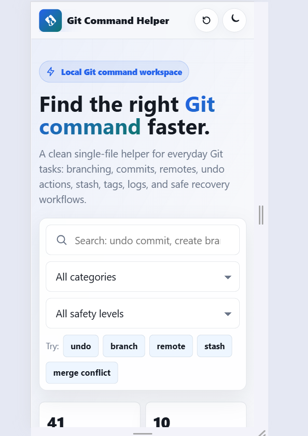
Show List

Time Series Analysis with Deep Learning

Time series analysis is a statistical technique that is used to analyze and model time series data, which is data that is collected over time. Deep learning models can be used for time series analysis, including forecasting and anomaly detection, by learning complex patterns and relationships in the data.

In this answer, I will provide a brief introduction to time series analysis with deep learning and some code examples using Python and TensorFlow, a popular deep learning library.

  • Preparing Time Series Data

The first step in any time series analysis task is to prepare the time series data. This typically involves splitting the data into training and testing sets, and normalizing the data to ensure that it has a consistent scale. Here's an example of how to prepare a time series dataset using the Air Passengers dataset:

python
Copy code
import pandas as pd from sklearn.preprocessing import MinMaxScaler # Load Air Passengers dataset url = 'https://raw.githubusercontent.com/jbrownlee/Datasets/master/airline-passengers.csv' df = pd.read_csv(url, header=0, index_col=0, parse_dates=True) # Split data into training and testing sets train_size = int(len(df) * 0.8) train_data, test_data = df.iloc[:train_size], df.iloc[train_size:] # Normalize data scaler = MinMaxScaler() train_data = scaler.fit_transform(train_data) test_data = scaler.transform(test_data)

In this code, we first load the Air Passengers dataset from a CSV file and split it into training and testing sets. We then normalize the data using the MinMaxScaler from scikit-learn to ensure that it has a consistent scale.

  • Building a Recurrent Neural Network Model

Once the time series data has been prepared, we can use it to train a deep learning model. In this example, we will build a recurrent neural network (RNN) model using TensorFlow to perform time series forecasting on the Air Passengers dataset.

python
Copy code
import tensorflow as tf from tensorflow.keras.models import Sequential from tensorflow.keras.layers import Dense, LSTM # Build LSTM model n_features = 1 timesteps = 12 model = Sequential() model.add(LSTM(50, input_shape=(timesteps, n_features))) model.add(Dense(1)) model.compile(optimizer='adam', loss='mse') # Reshape training and testing data X_train, y_train = train_data[:-timesteps], train_data[timesteps:] X_test, y_test = test_data[:-timesteps], test_data[timesteps:] X_train = X_train.reshape((X_train.shape[0], timesteps, n_features)) X_test = X_test.reshape((X_test.shape[0], timesteps, n_features)) # Train model batch_size = 32 epochs = 100 model.fit(X_train, y_train, batch_size=batch_size, epochs=epochs, validation_data=(X_test, y_test))

In this code, we first define the parameters for the LSTM model, including the number of features and timesteps. We then build an LSTM model with one hidden layer and compile it with the Adam optimizer and mean squared error loss. Finally, we reshape the training and testing data to have the required input shape for the LSTM model and train the model for 100 epochs.

  • Detecting Anomalies in Time Series Data

Another application of deep learning for time series analysis is anomaly detection, which involves identifying unusual or unexpected patterns in the data. One way to do this is to use an autoencoder, which is a type of neural network that is trained to reconstruct the input data with a bottleneck layer that forces the network to learn compressed representations of the data.

Here's an example of how to use an autoencoder for anomaly detection on the Yahoo S5 dataset


python
Copy code
import numpy as np import pandas as pd import matplotlib.pyplot as plt from sklearn.preprocessing import MinMaxScaler from tensorflow.keras.layers import Input, Dense, Dropout from tensorflow.keras.models import Model # Load Yahoo S5 dataset url = 'https://raw.githubusercontent.com/numenta/NAB/master/data/realKnownCause/nyc_taxi.csv' df = pd.read_csv(url, header=0, index_col=0, parse_dates=True) # Split data into training and testing sets train_size = int(len(df) * 0.8) train_data, test_data = df.iloc[:train_size], df.iloc[train_size:] # Normalize data scaler = MinMaxScaler() train_data = scaler.fit_transform(train_data) test_data = scaler.transform(test_data) # Build autoencoder model input_dim = train_data.shape[1] encoding_dim = 64 input_layer = Input(shape=(input_dim,)) encoder = Dropout(0.2)(Dense(encoding_dim, activation='relu')(input_layer)) decoder = Dropout(0.2)(Dense(input_dim, activation='sigmoid')(encoder)) autoencoder = Model(inputs=input_layer, outputs=decoder) autoencoder.compile(optimizer='adam', loss='mse') # Train model batch_size = 128 epochs = 50 history = autoencoder.fit(train_data, train_data, batch_size=batch_size, epochs=epochs, validation_data=(test_data, test_data)) # Detect anomalies in testing data threshold = np.mean(history.history['val_loss']) + np.std(history.history['val_loss']) predictions = autoencoder.predict(test_data) mse = np.mean(np.power(test_data - predictions, 2), axis=1) anomalies = test_data[mse > threshold] # Plot anomalies plt.plot(test_data) plt.plot(anomalies, 'ro') plt.show()

In this code, we first load the Yahoo S5 dataset from a CSV file and split it into training and testing sets. We then normalize the data using the MinMaxScaler and build an autoencoder model with one hidden layer and compile it with the Adam optimizer and mean squared error loss. Finally, we train the model for 50 epochs and use it to detect anomalies in the testing data based on a threshold calculated from the validation loss. We plot the original testing data and the detected anomalies for visualization.

Overall, deep learning has proven to be a powerful tool for time series analysis, with many applications in forecasting, anomaly detection, and other areas. By leveraging the ability of deep learning models to learn complex patterns and relationships in time series data, we can gain new insights and make more accurate predictions.


    Leave a Comment


  • captcha text